TFPIE2012: Recursion Schemes of Scientific Models

The Recursion Schemes of Scientific Models

By: Baltasar Trancón y Widemann

• Draft proceedings version File:TFPIE2012 Draft RecursionSchemesOfScientificModels Widemann.pdf
• Literate Haskell Archive File:TFPIE2012 Supplement RecursionSchemesOfScientificModels Widemann.zip

Visual Demonstrations

The following diagrams can be produced from the Literate Haskell code (provided some not quite hassle-free Haskell packages are installed, sorry).

• 

  Direct Modelling with Trajectories.
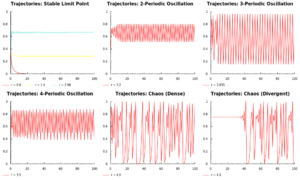
  Trajectories of the logistic map with different initial states and parameter values are plotted for 100 steps, showing six classes of behaviour. From top-left to bottom-right:
  1. Stable limit points that attract the initial state, either one-sided (<math>r<2</math>) or with overshooting (<math>r>2</math>). These correspond to the initial branch of the logistic map's bifurcation diagram.
  2. Stable periodic solution of period length 2 that attracts the initial state; corresponds to the first bifurcation at <math>r=3</math>.
  3. Stable periodic solution of period length 2 that attracts the initial state; more difficult to find in the bifurcation diagram in a small window of orderly behaviour among chaos.
  4. Stable periodic solution of period length 4 that attracts the initial state; corresponds to the second bifurcation at <math>r \approx 3.45</math>.
  5. Chaotic behaviour at <math>r = 4</math>, ranging over the whole domain. Illustrates one of the defining properties of chaos: orbits (points connected by a trajectory) are dense.
  6. Chaotic behaviour at <math>r = 4</math>, starting from a tiny neighbourhood of an unstable limit point. Illustrates another defining property of chaos: near trajectories diverge exponentially.

  The initial state is 0.35 in all cases except the last, where it is 0.7500000000001.

• 

  Direct Modelling with Intervals.
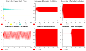
  The same six situations as above, but now with an interval of potential initial states. Note that periodic solutions are either self-focussing or self-dispersing, for one-sided and overshooting convergence, respectively. Note also how quickly the state becomes completely indeterminate when chaos emerges. The initial intervals are [0.3, 0.4] in all cases except the last, where it is [0.75, 0.7500000000001].
• 

  Inverse Modelling with Input.
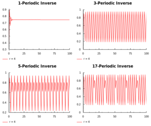
  Backwards trajectories for the logistic map with <math>r=4</math> are plotted for 100 steps. In the forward mode, the map is completely chaotic for this parameter value, i.e., periodic of all lengths exist, but are unstable. In the backwards mode, these solutions become stable such that most initial states are attracted to them. By the simple expedient of driving the reverse map with a periodic stream of binary input of the desired period length, convergence towards a solution of that period length is effected. Running forwards from a state obtained by this procedure, the appearance of a periodic trajectory is produced. Of course, it will break down eventually because of chaos, but the longer the backwards search procedure, the longer the appearance can be maintained. Simple cases of length 1 and 3 are shown, as well as for 5 and 17. Those are virtually impossible to construct in the forward mode.